Its been quite a while since my last post, and its Friday and I was
feeling creative, so I decided to map something! I’ve been looking for
an excuse to produce a nice graphic like the one Anita Graser
created to represent Vienna’s green-spaces. She used Quantum
GIS to produce a hexagonal grid for representing the density of
Viennese trees instead of the standard heat map or kernel density map,
and the results are quite nice! I’m a huge fan of QGIS, but I tend to do
most of my work in R, so I decided to see if I could produce something
similar using R. Turns out you can, and the final results are displayed
below (read on to see the full work-flow). Instead of trees, I went
ahead and mapped the locations of unique visitors to
http://www.carsonfarmer.com/ between 2009 and 2011:

Work-flow
Firstly, I downloaded the logs for www.carsonfarmer.com. I did this
directly from the console, though I’m pretty sure I could have done this
from R as well. Next, I needed to extract the unique IP addresses from
the logs. I found this nice grep one-liner from here, which I
modified to grab all unique IP addresses that ‘GET’ something from the site:
grep 'GET' access.log | cut -d' ' -f1 | sort | uniq > ip_addresses.log
To actually map the IP addresses, I obviously needed some way to convert the raw IP addresses to latitude and longitude coordinates. Enter the very nice Data Science Toolkit (DSTK) from Pete Warden and the very handy RDSTK R package from Ryan Elmore! Basically, the DSTK has an API that can be queried for all sorts of information useful for ‘data science’ applications, and the RDSTK makes it possible to query to API directly from within R. I first heard about both these projects from the Revolution Analytics blog, where there is an article summarising Ryan Elmore’s work on RDSTK, and a few other handy links. RDSTK isn’t (yet?) available on CRAN, so I downloaded it directly from github:
wget https://github.com/rtelmore/RDSTK/raw/master/src/RDSTK_1.0.tar.gz
Then I installed it via R CMD INSTALL (note that it requires other R
packages: RCurl, rjson, and plyr):
R CMD INSTALL RDSTK_1.0.tar.gz
Once I had all that stuff installed and ready to go, I actually started up an R session and got working:
addresses = read.table('ip_addresses.log', col.names='address')
library(RDSTK)
? ip2coordinates
The ip2coordinates function requires multiple IPs to be contained
within a single string with comma-separated IP addresses, but we can
only do a few IPs at a time (about 100 I think?) so I had to do this
part in a loop (it probably isn’t polite to slam DSTK with 1,000s of
requests, so be nice!).
ips = paste(as.character(addresses$address[1:80]), collapse=', ')
out = ip2coordinates(ips)
last = 80
s = c(seq(160, nrow(addresses), 80), nrow(addresses))
for (i in s) {
    ips = paste(as.character(addresses$address[(last+1):i]), collapse=', ')
    out = rbind(out, ip2coordinates(ips))
    last = i
}
Once that is done running, the next step(s) are to a) convert the
returned data.frame to a SpatialPointsDataFrame, b) create a
SpatialGrid based on the points, c) create a SpatialPolygons object
from a hexagonal sample of the grid, and then finally d) create a
SpatialPolygonsDataFrame for plotting:
library(sp)
# make the output into a Spatial* object
coordinates(out) = ~longitude+latitude
library(maptools) # need this for the following function
sg = Sobj_SpatialGrid(out, maxDim=200, n=NULL)$SG
hex_pts = spsample(sg, type='hexagonal', cellsize=sg@grid@cellsize)
hex_poly = HexPoints2SpatialPolygons(hex_pts)
pts_poly = over(hex_poly, out, returnList=TRUE)
pts_poly_count = sapply(pts_poly, function(x) nrow(x))
poly = SpatialPolygonsDataFrame(poly, data.frame('count'=pts_poly_count),
    match.ID=FALSE)
Ok, now for some plotting!
# pick some reasonable break points
breaks = c(1.0, 10.0, 20.0, 50.0, 100.0, 500.0, 2000.0)
# use RColorBrewer to get a nice blue palette
library(RColorBrewer)
# don't use the lightest colour, it looks washed out
cols = brewer.pal(7,"Blues")[-1]
# plot the grid, which produces something close to our final product
spplot(poly[poly$count>0,], col='white', col.regions=cols, at=breaks,
       par.settings=list(axis.line=list(col='transparent')))
I then used Inkscape to tweak the final product, adding titles and labels and modifying the colour key to look like something a bit more suited to the map at hand. In the end I had a nice map of my blog readers, and an excellent way to procrastinate on a sunny Friday afternoon!